Dashboards

Any data you write to a data store table can be rendered as a dashboard. No external warehouse, no separate BI tool, no schema migration — point a data source at the table, drop widgets on the canvas, and you have an interactive analytics view your team can filter, drill into, and export.

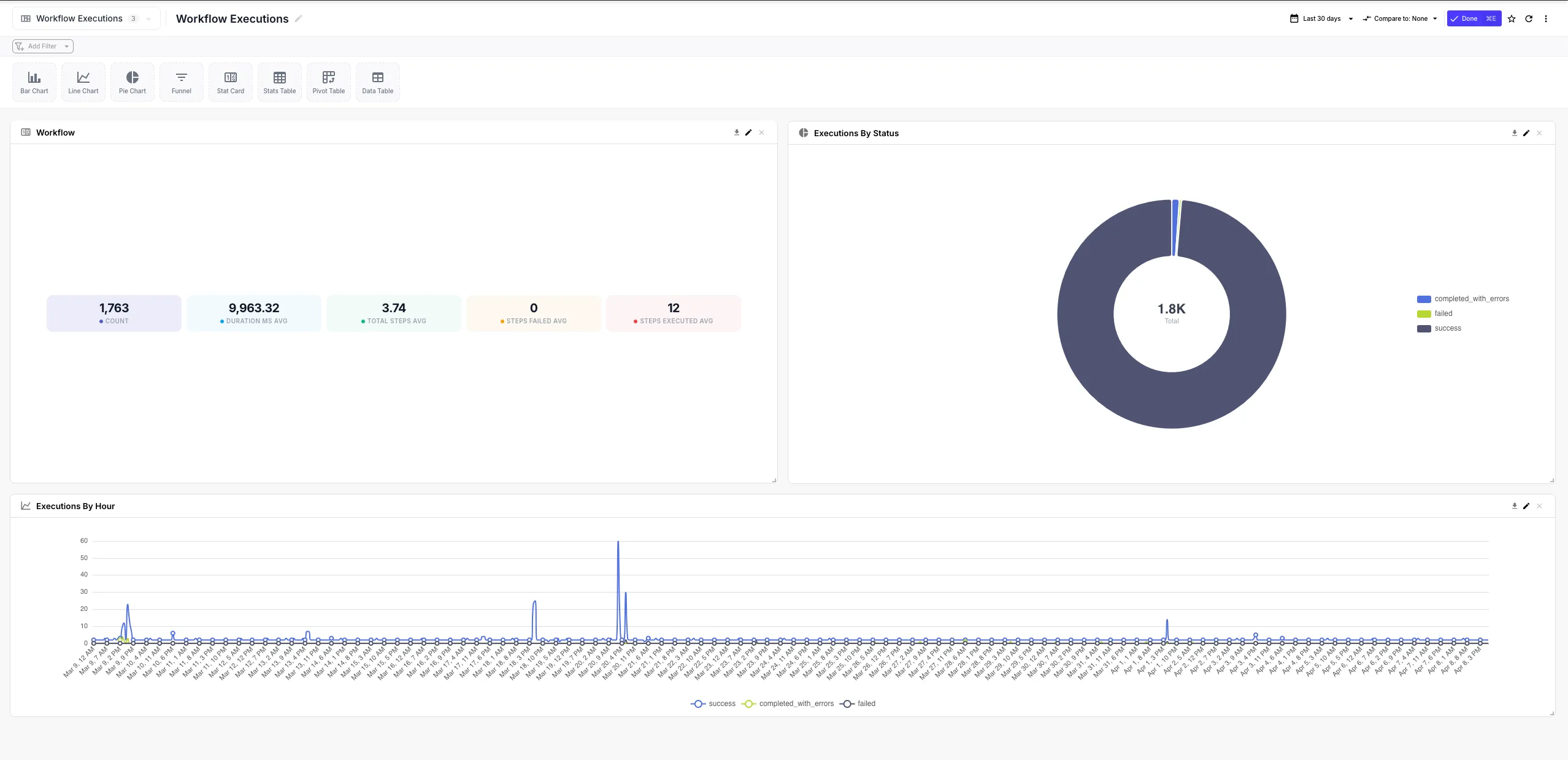
This is one of QuickFlo’s biggest force-multipliers: every workflow you build is already generating data that’s a few clicks away from being a dashboard. Log API call results to a data store, then chart them. Track pipeline conversions in a data store, then visualize them. Stream data from Five9 or your CRM into a data store, then build an executive dashboard on top — same workflow, same data, no extra moving parts.

How It Works

Dashboards have three building blocks:

Concept	What it is
Data Source	A pointer at a data store table, with a detected field schema and (optionally) a designated time field for date-range filtering. One data source can also aggregate multiple tables across organizations.
Widget	A chart, pivot table, stat card, data table, funnel, or pie that runs an analytics query against a data source — measures, dimensions, time range, filters, calculated fields.
Dashboard	A grid of widgets with shared filters, a date range selector, and a layout you can rearrange. Importable, exportable, and exportable to PDF.

The analytics engine reads directly from the data store tables you already have — no ETL job, no separate analytics database. Adding a data source takes seconds; the engine introspects the table on the fly and detects field types so the widget builders know what’s chartable, what’s filterable, and which field to use for time-series.

Quick Start

1. Have some data in a data store

   Any table in Data Stores works — written by your workflows, imported from a CSV, or shared into your org from a partner. If the table is empty you can still set it up; widgets just won’t have anything to render until rows arrive.

2. Add a Data Source

   From the Dashboards page, open Data Sources → Add Data Source. Pick your table from the dropdown (your own tables and any shared from other orgs are listed together). The dialog shows:

   • A preview of the most recent rows from the table
   • Detected fields with their types — string, number, boolean, or date — and a “chartable” badge on numeric fields the analytics engine can aggregate
   • A time filter field picker — click any date field to designate it as the dashboard’s date-range column
   

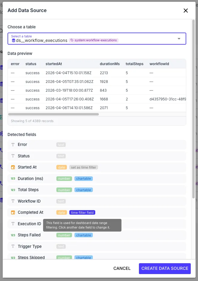
   Give the data source a name (e.g. “Production calls”) and click Create Data Source. You can repeat this to add as many data sources as you need.

3. Create a Dashboard

   From the Dashboards page, click New Dashboard and give it a name. You’ll land in the dashboard workspace with an empty canvas.

4. Add Widgets

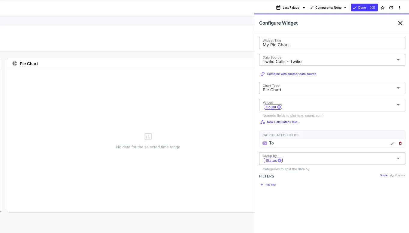
   Click Add Widget and pick a chart type from the palette. Choose your data source, then pick:

   • One or more measures (numeric fields to aggregate — the engine offers count, sum, avg, min, max automatically)
   • Zero or more dimensions (string/categorical fields to group by)
   • An optional time dimension (the date field you set when creating the data source) with a granularity (15 min / hour / day / week / month / year)
   • Optional filters to narrow the data
   • An optional time range (last 24h, 7d, 30d, 90d, or a custom absolute range)
   

   The widget renders immediately. Drag it to position it on the grid; resize from the corner.

5. Add Filters

   Hit + Filter in the dashboard toolbar to add a top-level filter — pick a dimension from any data source and label it. Filters can auto-wire to multiple data sources at once, so a single “Region” dropdown can drive every widget on the page in one go (see Filters below).

That’s it. Anything you do later — adding more widgets, sharing the dashboard with another org, exporting as JSON for version control — builds on these same primitives.

Data Sources

A data source is a thin wrapper around a data store table:

Field	Description
Name	A human-readable label shown in the widget builder
Table	The underlying data store table the data source reads from
Detected schema	Fields with their types and which ones are aggregatable
Time dimension	The date field used for dashboard date-range filtering (set during creation, changeable later)
Sync config	Optional — if the data source is populated by a recurring sync workflow, the schedule and last-sync status are surfaced here

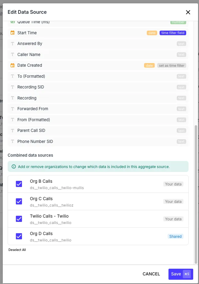
Aggregating Multiple Tables

A single data source can aggregate multiple tables across organizations — useful for partner or multi-tenant scenarios where you want to chart “all customer call volume” without picking one tenant at a time. When you select an additional table during data source creation, the analytics engine reads from each table’s organization in turn and exposes a virtual _customer dimension you can group/filter on. Rows from the underlying tables are tagged with whichever alias you give each entry.

Aggregate sources work for both:

• Cross-org aggregation — your own table plus tables shared from partner organizations (see Sharing Tables Across Organizations)
• Same-org multi-table aggregation — your own table combined with other tables in your own org

Shared Data Sources

A data source can also point at just a table that was shared into your org by another organization. In that case the data source appears in the picker with a “Shared” badge and reads from the partner’s data while still living in your own dashboards. Revoking the share immediately stops new queries against the data source — any widget backed by it surfaces a clear error inline.

Widgets

Each widget runs an analytics query and renders a chart. Available widget types:

Widget	Best for
Bar	Comparing measures across categories
Line / Area	Trends over time
Pie / Doughnut	Share-of-total breakdowns (use sparingly — bars are usually clearer)
Stat Card	A single headline number (with optional comparison delta)
Funnel	Multi-stage conversion flow
Data Table	Raw rows or grouped detail with sortable columns
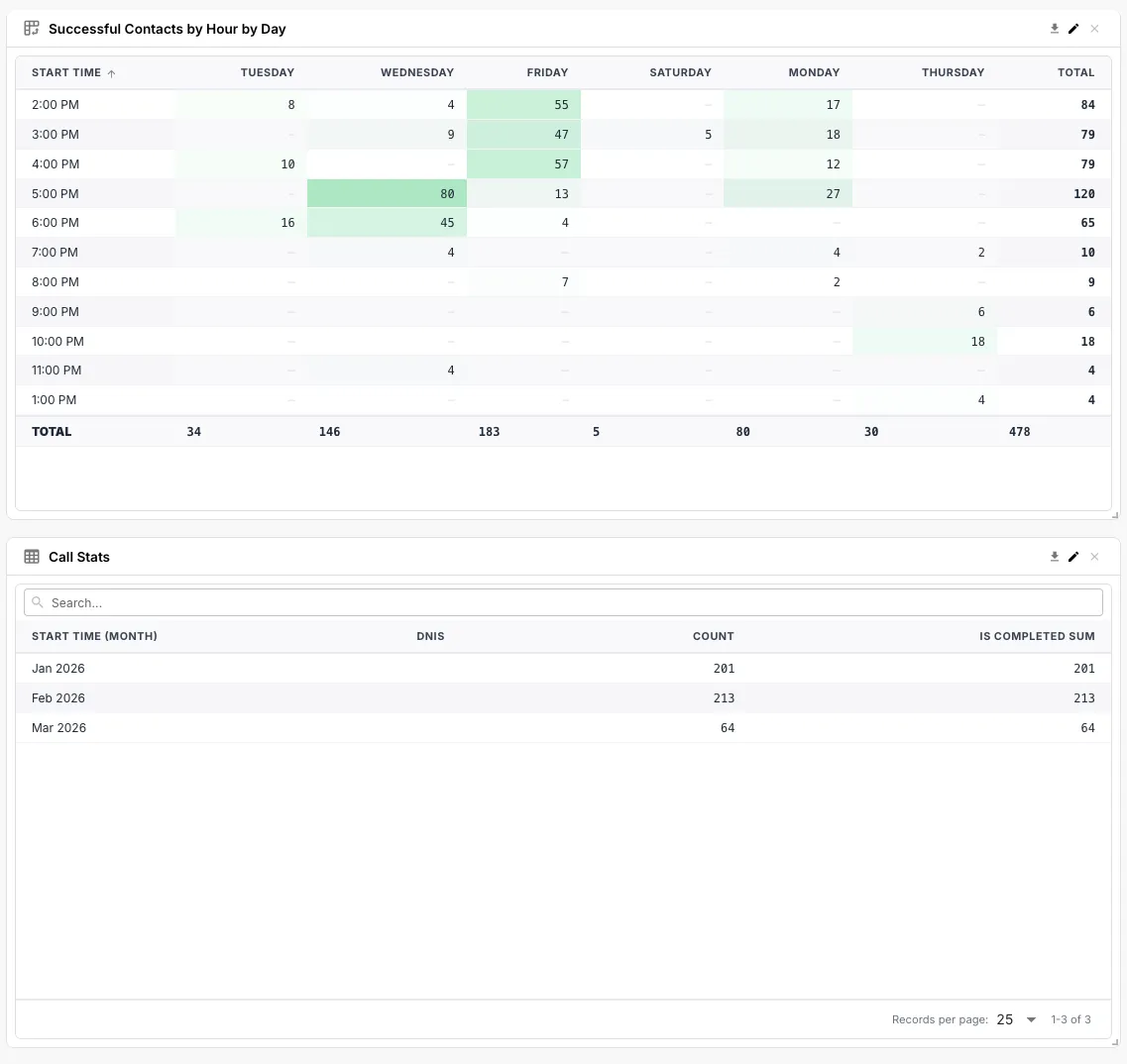
Stats Table	A grid of measures × categories — like a multi-column stat card
Pivot Table	Two-dimensional grid with row/column dimensions, ratio mode, and heatmap shading

Query Configuration

Every widget has the same query shape under the hood:

• Measures — what to aggregate (e.g. count, sum(amount), avg(durationSeconds))
• Dimensions — what to group by (e.g. region, direction, agentName)
• Time dimensions — a date field plus a granularity (15min, 30min, hour, day, week, month, year)
• Filters — narrow the dataset before aggregation
• Joins — optionally join in another data source by a key field
• Order — sort the result set by a measure or dimension
• Limit — cap the number of rows returned
• Time range — the date window the query covers (relative last 7 days, or an absolute start/end)

Pivot Tables

The pivot table widget supports:

• Row and column dimensions — including inline date bucketing via field suffixes (createdAt:hourOfDay, createdAt:dayOfWeek, createdAt:month, etc.) so you can pivot “calls by agent × hour of day” without precomputing the bucket
• Ratio mode — switch the cell display from raw measure values to ratios (with percent formatting) for “what fraction of the total” views
• Heatmap shading — color-scale cells from low to high so outliers pop visually

Filters

Dashboards have two layers of filtering:

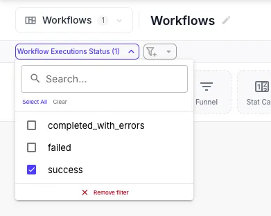
Dashboard-Level Filters (Auto-Wire)

Click + Filter in the dashboard toolbar to add a global filter that drives the whole dashboard — a region dropdown, a customer selector, an environment switcher. Each filter has:

• A label shown in the toolbar
• Bindings — one or more (data source, dimension) pairs that this filter targets

The bindings array is the magic: a single filter can wire itself to multiple data sources at once by mapping the same logical concept (region) to whichever field name each data source uses for it. Add a “Region” filter, bind it to region on data source A and geography.region_code on data source B, and selecting “EMEA” updates every widget connected to either source. No widget changes needed.

You can save default filter selections so a dashboard always loads with a sensible starting state.

Widget-Level Filters

Each widget can also have its own filters, applied on top of the dashboard’s. These come in two flavours:

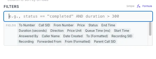
• Simple mode — structured rows with field, operator, and value (status equals active, amount greater than 100). Operators are equals, notEquals, contains, notContains, gt (>), gte (>=), lt (<), lte (<=), set (is set), and notSet (is not set). The equals and notEquals operators support multi-value chip selection with searchable options pulled from the underlying data, so you can pick a list of accepted values without typing them by hand.
• Formula mode — a code editor for complex expressions in JavaScript-style syntax (operators like ==, !=, &&, ||, comparison, arithmetic, member access, function calls — see jsep for the full grammar reference), with reference pills for fields and live syntax highlighting. Use this when simple rows don’t cut it — for example (status == 'active' OR retryCount > 3) AND createdAt > '2024-01-01'.

Calculated Fields

Sometimes you need a value that doesn’t live in your raw data — a margin computed from cost and revenue, a duration from two timestamps, a category derived from a string match. Calculated fields let you define these as formula expressions on the data source, and the analytics engine compiles them to SQL at query time.

The CalculatedField builder gives you:

• A CodeMirror formula editor with syntax highlighting
• Reference pills — click any existing field to insert it into the formula
• Quick-start templates for common patterns (margin %, duration in seconds, conditional bucketing)

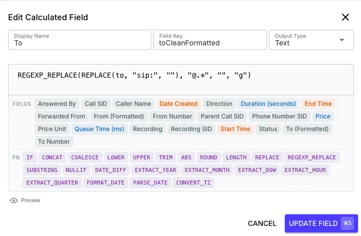
Once defined, the calculated field appears in the widget builder alongside native fields — you can use it as a measure, dimension, or filter just like any other column. Formulas use JavaScript-style expression syntax (jsep grammar) and are compiled to SQL at query time, so they execute server-side without pulling rows back to render.

Drill-Downs

Click into any aggregated cell — a bar, a pie slice, a stat card, a pivot cell, a stats-table row — and a full-screen drill-down dialog opens showing the raw underlying records that contributed to that aggregate. Bar, line, pie, stat card, stats table, and pivot table widgets all support it; data tables don’t (they’re already showing rows) and funnels don’t either.

The dialog renders a data-table view containing every field from the underlying data source, with the click’s filters applied automatically — so the rows are scoped to whatever you clicked. The dashboard’s global filters and date range carry through too, so the drill-down always reflects the same slice you were looking at on the page.

Importing & Exporting Dashboards

Dashboards are JSON. Export one, commit it to git, share it with a teammate, paste it into another QuickFlo organization — same dashboard, ready to go.

Export

From any dashboard’s menu, choose Export to download a .json file. The export contains:

• The dashboard’s layout, name, description, and filter config
• Every widget’s query config and display config with internal data source IDs replaced by stable export-only aliases (ds-0, ds-1, …)
• A schema fingerprint for each referenced data source so the importer can detect compatibility issues when remapping

Exports are intentionally not backed by the underlying rows — only the dashboard definition travels with the file. The data stays in whichever data store the partner is targeting on the import side.

Import

From the Dashboards page, click Import Dashboard and drop in a .json file. The import dialog walks you through two phases:

1. Upload — drag in the file. QuickFlo parses it and surfaces any structural errors before showing you the next phase.

2. Map data sources — for each data source the export references, pick one of your data sources to map it to. Each option shows a compatibility badge based on how well its detected schema matches the export’s schema fingerprint, so you can quickly spot which mapping is the safe one.

   

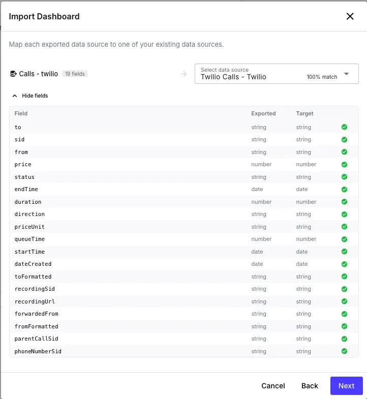
Click Import and QuickFlo creates a fresh dashboard in your org with all the widgets, filters, and layout intact — every data source reference, calculated field expression, and filter binding rewritten to point at the data sources you mapped.

This makes dashboards highly portable — you can build a “starter” dashboard once and ship it to every customer organization, or version-control your important dashboards alongside the rest of your codebase.

PDF Export

Beyond JSON export, you can also render any dashboard to a PDF for sharing with stakeholders who don’t have QuickFlo access. The PDF preserves widget rendering, layout, and the active filter state at the moment you exported, so the PDF is a frozen snapshot of what you were looking at on screen.

Sharing Dashboards Across Organizations

Cross-org sharing is built at the data store layer rather than the dashboard layer — you grant another organization read-only access to a specific data store table, and the partner builds their own dashboards on top of it. See Data Stores — Sharing Tables Across Organizations for the setup walkthrough.

The end result feels seamless from the partner’s side: they add a data source, the shared table appears in the picker with a “Shared” badge, and dashboards built on it work exactly like dashboards on their own data — including filters, calculated fields, drill-downs, and exports.

Tip

Pair shared tables with dashboard import/export to ship a complete partner experience: share the data store, send the partner a dashboard .json file, and they import it and map the data source in two clicks. Done.